ML Feature Pipeline

varistar.ml turns a collection of (TimeSeries, LightCurve) pairs into a feature matrix, then clusters it. Dataset is the interactive entry point; FeaturePipeline is the CLI equivalent for a directory of .dat files.

from varistar import TimeSeries, LightCurve
from varistar.ml.data import Dataset
from _synthetic import make_sinusoidal_lightcurve, make_eclipsing_lightcurve

ds = Dataset(data_dir="./_scratch")  # only used if you later call export_features()

for i in range(4):
    df = make_sinusoidal_lightcurve(period=1.5 + 0.4 * i, seed=100 + i)
    ts = TimeSeries(magnitude="mag I", time_scale="HJD")
    ts.load_data_from_df(df, data_id=f"sine_{i:02d}")
    ds.add_object(ts, LightCurve(ts))

for i in range(4):
    df = make_eclipsing_lightcurve(period=3.0 + 0.5 * i, seed=200 + i)
    ts = TimeSeries(magnitude="mag I", time_scale="HJD")
    ts.load_data_from_df(df, data_id=f"eb_{i:02d}")
    ds.add_object(ts, LightCurve(ts))

len(ds)

Feature extraction

18 statistical and astrophysical features per star (n_cores=1 here so docs builds stay deterministic and single-process; raise it for real datasets):

features = ds.build_features(n_cores=1)
features.head()

Extracting 18 features for 8 stars using 1 worker(s)...

Features:   0%|          | 0/8 [00:00<?, ?it/s]
Features:  12%|█▎        | 1/8 [00:01<00:11,  1.63s/it]
Features: 100%|██████████| 8/8 [00:01<00:00,  4.77it/s]

Done. Feature matrix shape: (8, 18)

	median	mad	octile_skew	low	row	mav	skew	stetson_j	flux_perc_ratio	log_freq	log_amp	r21	ph21_cos	ph21_sin	freq_ratio	von_neumann	kurtosis	beyond1std
id
sine_00	14.951740	0.166829	0.189136	0.193654	0.240996	0.348094	0.201077	0.309150	3.281441	-0.175862	-0.240124	0.006874	0.660781	-0.750578	0.998747	1.288633	-1.449550	0.472500
sine_01	15.022269	0.183528	-0.098277	0.213774	0.162972	0.222661	-0.099757	0.474463	3.279984	-0.278745	-0.232032	0.003478	0.551693	-0.834047	0.998408	0.921233	-1.496527	0.510000
sine_02	14.977564	0.167837	0.078717	0.192879	0.237459	0.227769	0.098007	0.503178	3.471829	-0.362145	-0.246232	0.012902	0.999299	0.037447	1.001941	0.872591	-1.432720	0.485000
sine_03	14.990327	0.168094	0.033304	0.258124	0.251973	0.185170	0.024304	0.575821	3.709217	-0.430923	-0.239747	0.003099	0.721878	-0.692020	0.997723	0.697706	-1.407703	0.467500
eb_00	14.516083	0.026262	0.787165	0.355746	0.492507	3.098591	1.870418	0.318536	25.579643	-0.175760	-0.180594	0.671235	-0.022895	-0.999738	0.998996	1.194360	2.583707	0.121667

A single object’s features, without a Dataset:

from varistar.ml.features import FeatureExtractor

FeatureExtractor.extract(ts_obj=ts, lc_obj=LightCurve(ts))

{'id': 'eb_03',
 'median': 14.513510845943607,
 'mad': 0.0231098868662869,
 'octile_skew': 0.8102747606539833,
 'low': 0.3426635039358418,
 'row': 0.6915083175115532,
 'mav': 2.5723796625588657,
 'skew': 2.0290688803683263,
 'stetson_j': 0.44216469327519986,
 'flux_perc_ratio': 30.411516136791843,
 'log_freq': -0.3524273582841337,
 'log_amp': -0.18215504515974948,
 'r21': 0.7156677153912228,
 'ph21_cos': 0.018359270416665654,
 'ph21_sin': -0.9998314543910727,
 'freq_ratio': 1.001504900047014,
 'von_neumann': 0.7911990804613463,
 'kurtosis': 3.0893407150292695,
 'beyond1std': 0.13166666666666665}

Clustering

ds.cluster_data(n_clusters=2)
ds.visualize_clusters()

K-Means complete. Cluster distribution: {0: 4, 1: 4}

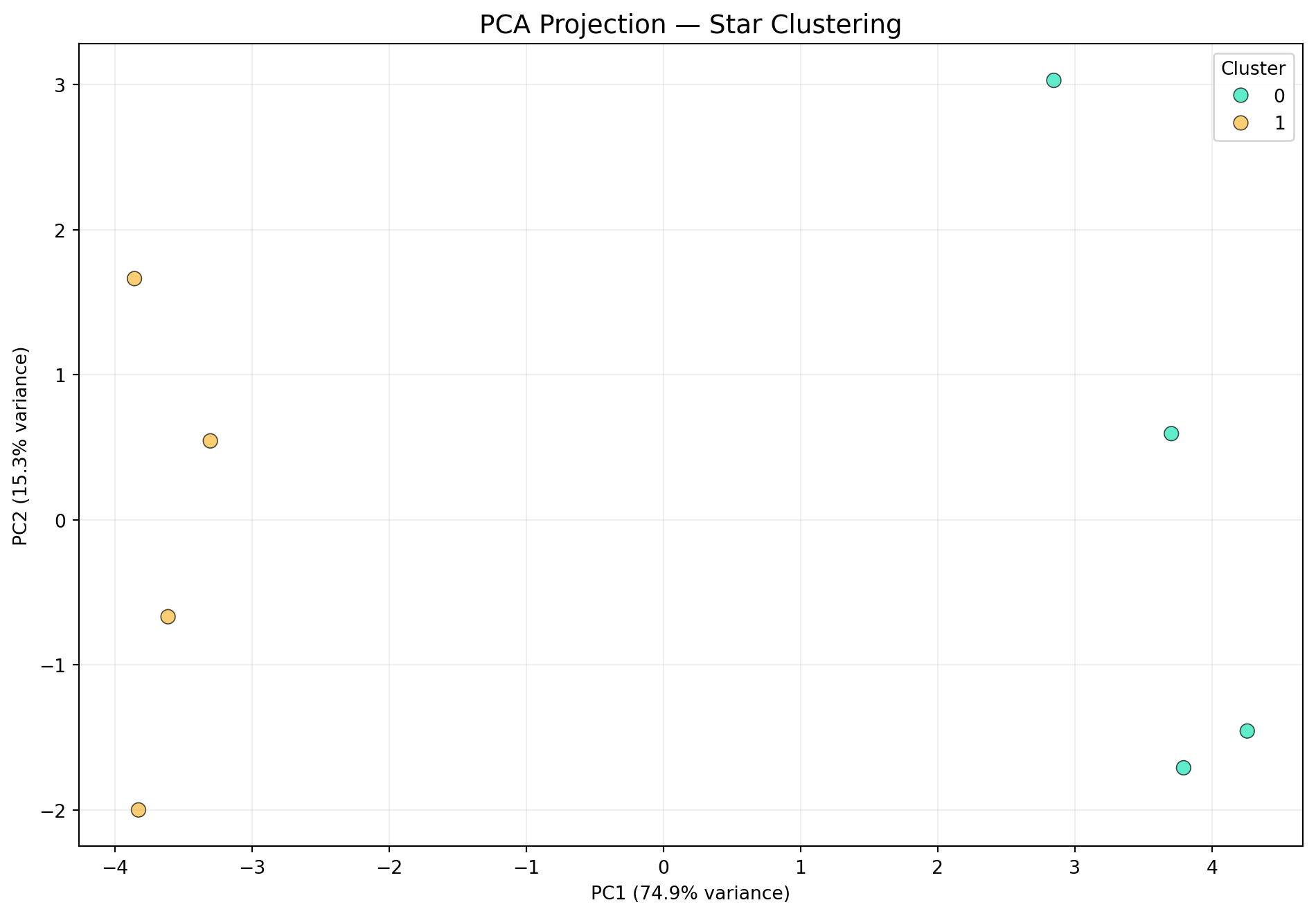
Top 5 features driving PC1 separation:
median        0.271079
r21           0.270773
beyond1std    0.270707
mad           0.270554
skew          0.270445

CLI: whole directories of `.dat` files

For a real survey field, skip the Python loop and run the pipeline directly against a directory (illustrative — not executed on this page):

python -m varistar.ml.pipeline --data ./ogle_field_01/ \
  --features 0 1 7 11 15 --output ./catalogues/

Next: Visualization.

Feature extraction​

Clustering​

CLI: whole directories of .dat files​

Feature extraction

Clustering

CLI: whole directories of `.dat` files